Predicting chocolate bar ratings
By Alex Labuda
November 26, 2022
In this post, we will be predicting chocolate bar ratings based on a variety of features
The Data
The data includes various chocolate bars and their corresponding ratings
tuesdata <- tidytuesdayR::tt_load(2022, week = 3)
##
## 	Downloading file 1 of 1: `chocolate.csv`
chocolate <- tuesdata$chocolate
Explore data
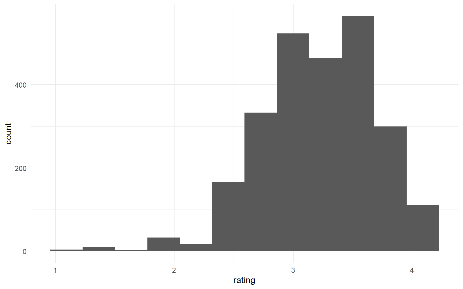
First we’ll start by exploring the data
Exploratory data analysis (EDA) is an important part of the modeling process.
chocolate %>%
  ggplot(aes(rating)) +
  geom_histogram(bins = 12)
Next I will replace missing values in ingredients with the most common ingredient and remove % from cocoa_percent column
chocolate <-
  chocolate %>%
  mutate(
    ingredients = replace_na(ingredients, "3- B,S,C")
    )

chocolate <-
  chocolate %>%
  mutate(cocoa_percent = as.integer(str_remove_all(cocoa_percent, "%")))
Next I bin all infrequent ingredients, company_location and country_of_bean_origin in “Other” category
chocolate <-
  chocolate %>%
  mutate(
    ingredients = ifelse(!ingredients %in% c("3- B,S,C", "2- B,S"),
                         "Other",
                         ingredients),
    company_location = ifelse(!company_location %in% c("U.S.A.", "Canada", "France",
                                                       "U.K.", "Italy", "Belgium"),
                              "Other",
                              company_location),
    country_of_bean_origin = ifelse(!country_of_bean_origin %in% c("Venezuela", "Peru",
                                                                   "Dominican Republic",
                                                                   "Ecuador", "Madagascar",
                                                                   "Blend", "Nicaragua"),
                                    "Other",
                                    country_of_bean_origin)
  )
Now we can preview out data with skimr::skim()
skimr::skim(chocolate)
Table: Table 1: Data summary
| Name | chocolate |
| Number of rows | 2530 |
| Number of columns | 10 |
| _______________________ | |
| Column type frequency: | |
| character | 6 |
| numeric | 4 |
| ________________________ | |
| Group variables | None |
Variable type: character
| skim_variable | n_missing | complete_rate | min | max | empty | n_unique | whitespace |
|---|---|---|---|---|---|---|---|
| company_manufacturer | 0 | 1 | 2 | 39 | 0 | 580 | 0 |
| company_location | 0 | 1 | 4 | 7 | 0 | 7 | 0 |
| country_of_bean_origin | 0 | 1 | 4 | 18 | 0 | 8 | 0 |
| specific_bean_origin_or_bar_name | 0 | 1 | 3 | 51 | 0 | 1605 | 0 |
| ingredients | 0 | 1 | 5 | 8 | 0 | 3 | 0 |
| most_memorable_characteristics | 0 | 1 | 3 | 37 | 0 | 2487 | 0 |
Variable type: numeric
| skim_variable | n_missing | complete_rate | mean | sd | p0 | p25 | p50 | p75 | p100 | hist |
|---|---|---|---|---|---|---|---|---|---|---|
| ref | 0 | 1 | 1429.80 | 757.65 | 5 | 802 | 1454.00 | 2079.0 | 2712 | ▆▇▇▇▇ |
| review_date | 0 | 1 | 2014.37 | 3.97 | 2006 | 2012 | 2015.00 | 2018.0 | 2021 | ▃▅▇▆▅ |
| cocoa_percent | 0 | 1 | 71.64 | 5.62 | 42 | 70 | 70.00 | 74.0 | 100 | ▁▁▇▁▁ |
| rating | 0 | 1 | 3.20 | 0.45 | 1 | 3 | 3.25 | 3.5 | 4 | ▁▁▅▇▇ |
Feature Engineering
Here we will unnest each word in most_memorable_characteristics and examine. We will then use these in our predictions
library(tidytext)

tidy_chocolate <-
  chocolate %>%
  # puts each word on it's own row
  unnest_tokens(word, most_memorable_characteristics)

tidy_chocolate %>%
  count(word, sort = TRUE)
## # A tibble: 547 × 2
##    word        n
##    <chr>   <int>
##  1 cocoa     419
##  2 sweet     318
##  3 nutty     278
##  4 fruit     273
##  5 roasty    228
##  6 mild      226
##  7 sour      208
##  8 earthy    199
##  9 creamy    189
## 10 intense   178
## # … with 537 more rows
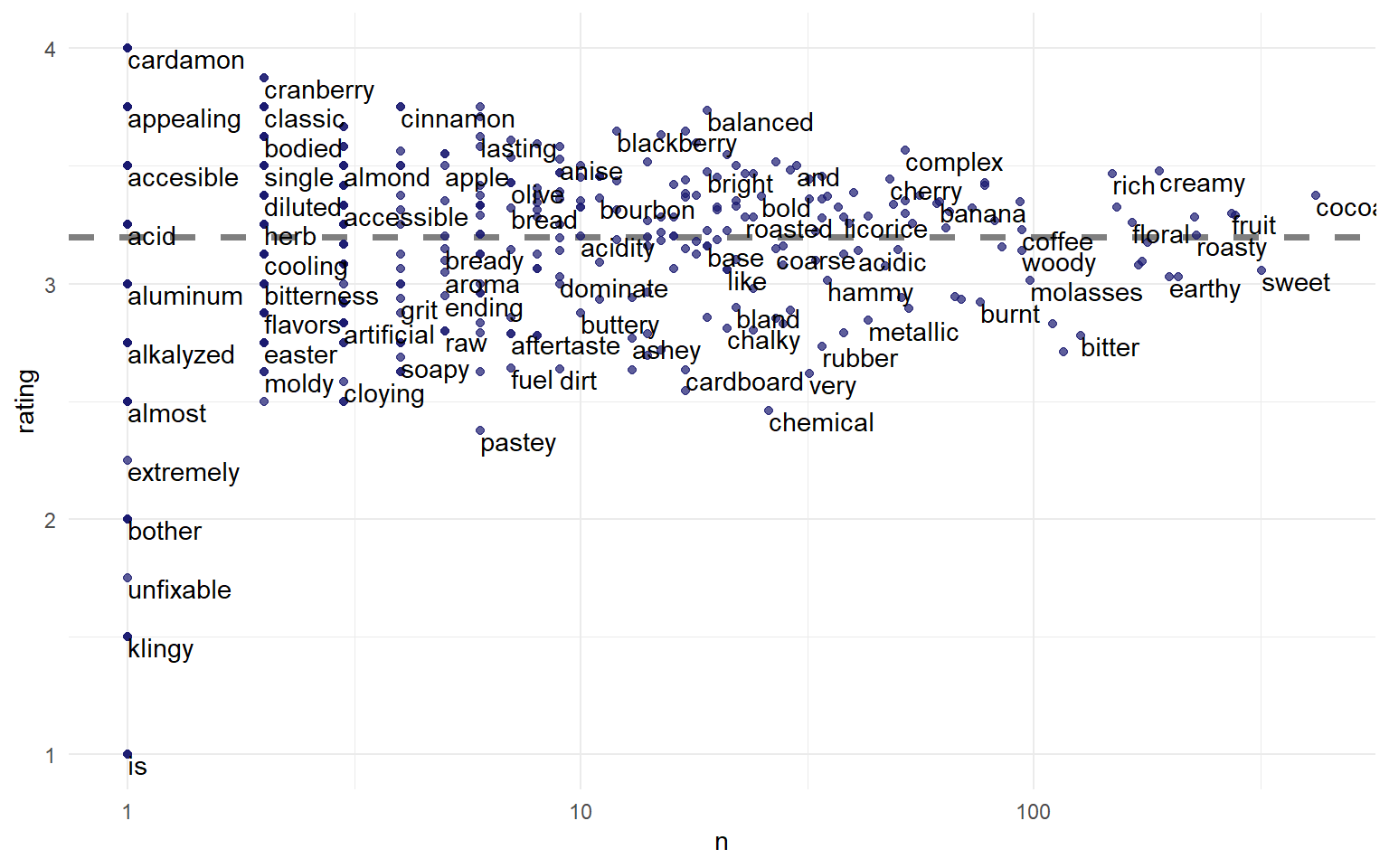
Rating by word count
We can examine most common words in this field
tidy_chocolate %>%
  group_by(word) %>%
  summarise(n = n(),
            rating = mean(rating)) %>%
  ggplot(aes(n, rating)) +
  geom_hline(yintercept = mean(chocolate$rating),
             lty = 2, color = "gray50", size = 1.25) +
  geom_point(color = "midnightblue", alpha = 0.7) +
  geom_text(aes(label = word),
            check_overlap = TRUE, vjust = "top", hjust = "left") +
  scale_x_log10()
Build models
Let’s consider how to spend our data budget:
- create training and testing sets
- create resampling folds from the training set
library(tidymodels)
## ── Attaching packages ────────────────────────────────────── tidymodels 1.0.0 ──
## ✔ broom        1.0.1          ✔ rsample      1.1.0
## ✔ dials        1.0.0.9000     ✔ tune         1.0.0
## ✔ infer        1.0.3          ✔ workflows    1.1.0
## ✔ modeldata    1.0.1          ✔ workflowsets 1.0.0
## ✔ parsnip      1.0.2          ✔ yardstick    1.1.0
## ✔ recipes      1.0.1
## ── Conflicts ───────────────────────────────────────── tidymodels_conflicts() ──
## ✖ scales::discard() masks purrr::discard()
## ✖ dplyr::filter()   masks stats::filter()
## ✖ recipes::fixed()  masks stringr::fixed()
## ✖ dplyr::lag()      masks stats::lag()
## ✖ yardstick::spec() masks readr::spec()
## ✖ recipes::step()   masks stats::step()
## • Learn how to get started at https://www.tidymodels.org/start/
set.seed(123)
choco_split <- initial_split(chocolate, strata = rating)
choco_train <- training(choco_split)
choco_test <- testing(choco_split)

set.seed(234)
choco_folds <- vfold_cv(choco_train, strata = rating)
choco_folds
## #  10-fold cross-validation using stratification
## # A tibble: 10 × 2
##    splits             id
##    <list>             <chr>
##  1 <split [1705/191]> Fold01
##  2 <split [1705/191]> Fold02
##  3 <split [1705/191]> Fold03
##  4 <split [1706/190]> Fold04
##  5 <split [1706/190]> Fold05
##  6 <split [1706/190]> Fold06
##  7 <split [1707/189]> Fold07
##  8 <split [1707/189]> Fold08
##  9 <split [1708/188]> Fold09
## 10 <split [1709/187]> Fold10
Preprocessing
Let’s set up our preprocessing
Recipe
library(textrecipes)

choco_recipe <-
  # recipe for the estimator
  recipe(rating ~ most_memorable_characteristics
         , data = choco_train) %>%
  # steps to build the estimator
  step_tokenize(most_memorable_characteristics) %>%
  step_tokenfilter(most_memorable_characteristics, max_tokens = 100) %>%
  step_tf(most_memorable_characteristics)


# Next steps are not necessary here, but are good to take a look at whats going on

# prep on recipe is analogous with fit on a model
# now the steps say [trained]
prep(choco_recipe)
## Recipe
##
## Inputs:
##
##       role #variables
##    outcome          1
##  predictor          1
##
## Training data contained 1896 data points and no missing data.
##
## Operations:
##
## Tokenization for most_memorable_characteristics [trained]
## Text filtering for most_memorable_characteristics [trained]
## Term frequency with most_memorable_characteristics [trained]
# bake for a recipe is like predict for a model
prep(choco_recipe) %>%
  bake(new_data = NULL)
## # A tibble: 1,896 × 101
##    rating tf_most_memo…¹ tf_mo…² tf_mo…³ tf_mo…⁴ tf_mo…⁵ tf_mo…⁶ tf_mo…⁷ tf_mo…⁸
##     <dbl>          <dbl>   <dbl>   <dbl>   <dbl>   <dbl>   <dbl>   <dbl>   <dbl>
##  1   3                 0       0       0       0       0       0       0       0
##  2   2.75              0       0       0       0       0       0       0       0
##  3   3                 0       0       0       0       0       0       0       0
##  4   3                 0       0       0       0       0       0       0       0
##  5   2.75              0       0       0       0       0       0       0       0
##  6   3                 1       0       0       0       0       0       0       0
##  7   2.75              0       0       0       0       0       0       0       0
##  8   2.5               0       0       0       0       0       0       0       0
##  9   2.75              0       0       0       0       0       0       0       0
## 10   3                 0       0       0       0       0       0       0       0
## # … with 1,886 more rows, 92 more variables:
## #   tf_most_memorable_characteristics_black <dbl>,
## #   tf_most_memorable_characteristics_bland <dbl>,
## #   tf_most_memorable_characteristics_bold <dbl>,
## #   tf_most_memorable_characteristics_bright <dbl>,
## #   tf_most_memorable_characteristics_brownie <dbl>,
## #   tf_most_memorable_characteristics_burnt <dbl>, …
Specs
Let’s create a model specification for each model we want to try:
ranger_spec <-
  # the algorithm
  rand_forest(trees = 500) %>%
  # engine (computation to fit the model (keras, spark, etc.))
  set_engine("ranger") %>% # range is the default
  # describes the modeling problem you're working with (regression, classification, etc.)
  set_mode("regression")

ranger_spec
## Random Forest Model Specification (regression)
##
## Main Arguments:
##   trees = 500
##
## Computational engine: ranger
svm_spec <-
  svm_linear() %>%
  set_engine("LiblineaR") %>%
  set_mode("regression")

svm_spec
## Linear Support Vector Machine Model Specification (regression)
##
## Computational engine: LiblineaR
To set up your modeling code, consider using the parsnip addin or the usemodels package.
Now let’s build a model workflow combining each model specification with a data preprocessor:
WorkFlow
# we're using a workflow bc we have a more complex model preprocess
ranger_wf <- workflow(choco_recipe, ranger_spec)
svm_wf <- workflow(choco_recipe, svm_spec)
If your feature engineering needs are more complex than provided by a formula like sex ~ ., use a
recipe.
Read more about feature engineering with recipes to learn how they work.
Evaluate models
These models have no tuning parameters so we can evaluate them as they are. Learn about tuning hyperparameters here.
doParallel::registerDoParallel()
contrl_preds <- control_resamples(save_pred = TRUE) # keep predictions

svm_rs <- fit_resamples(
  svm_wf,
  resamples = choco_folds,
  control = contrl_preds
)

ranger_rs <- fit_resamples(
  ranger_wf,
  resamples = choco_folds,
  control = contrl_preds
)
How did these two models compare?
collect_metrics(svm_rs)
## # A tibble: 2 × 6
##   .metric .estimator  mean     n std_err .config
##   <chr>   <chr>      <dbl> <int>   <dbl> <chr>
## 1 rmse    standard   0.348    10 0.00704 Preprocessor1_Model1
## 2 rsq     standard   0.365    10 0.0146  Preprocessor1_Model1
collect_metrics(ranger_rs)
## # A tibble: 2 × 6
##   .metric .estimator  mean     n std_err .config
##   <chr>   <chr>      <dbl> <int>   <dbl> <chr>
## 1 rmse    standard   0.344    10 0.00715 Preprocessor1_Model1
## 2 rsq     standard   0.379    10 0.0151  Preprocessor1_Model1
We can visualize these results:
bind_rows(
  collect_predictions(svm_rs) %>%
    mutate(mod = "SVM"),
  collect_predictions(ranger_rs) %>%
    mutate(mod = "ranger")
) %>%
  ggplot(aes(rating, .pred, color = id)) +
  geom_abline(lty = 2, color = "gray50", size = 1.2) +
  geom_jitter(width = 0.5, alpha = 0.5) +
  facet_wrap(vars(mod)) +
  coord_fixed()
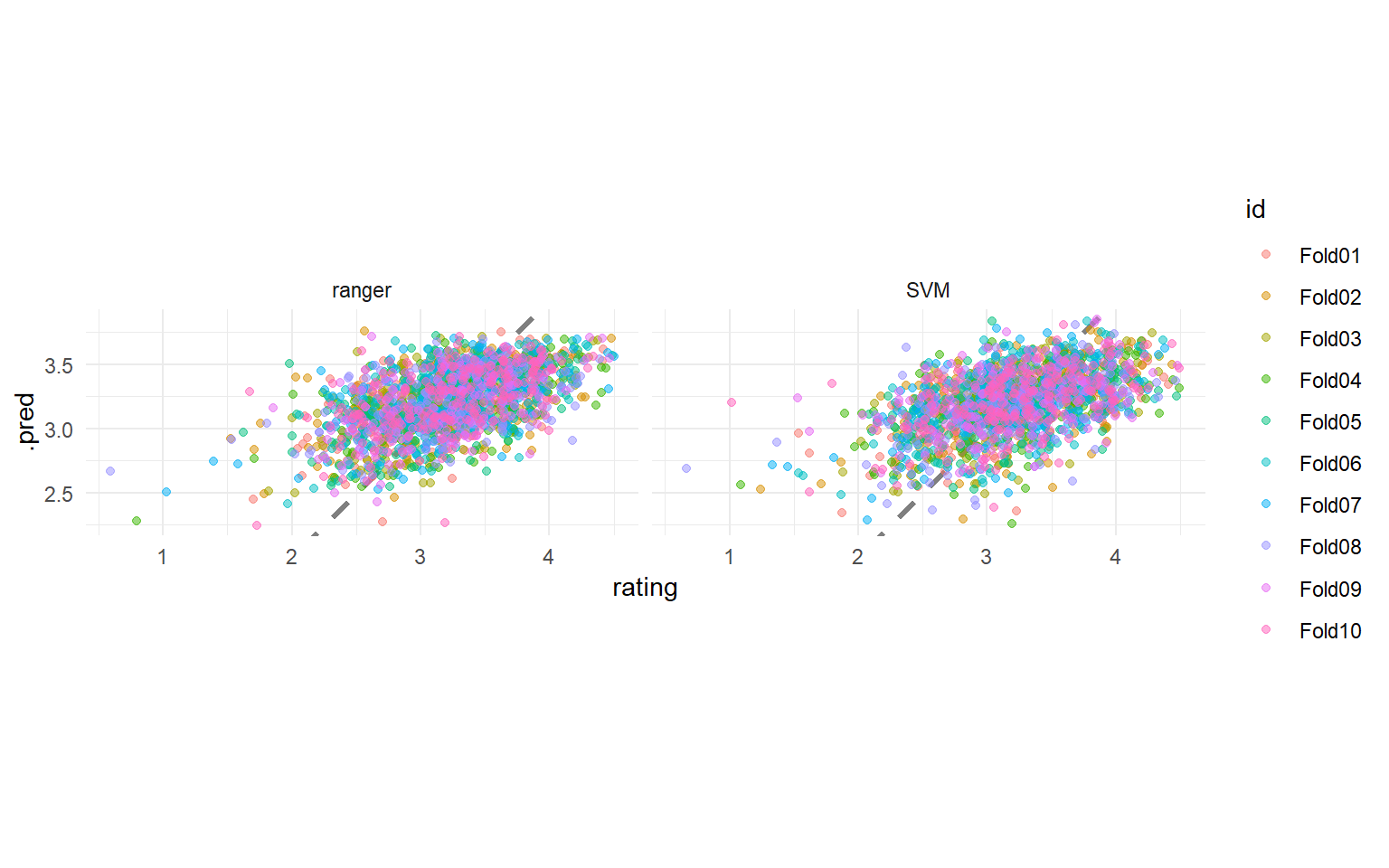
These models perform very similarly, so perhaps we would choose the simpler, linear model. The function last_fit() fits one final time on the training data and evaluates on the testing data. This is the first time we have used the testing data.
final_fitted <- last_fit(svm_wf, choco_split)
collect_metrics(final_fitted)  ## metrics evaluated on the *testing* data
## # A tibble: 2 × 4
##   .metric .estimator .estimate .config
##   <chr>   <chr>          <dbl> <chr>
## 1 rmse    standard       0.385 Preprocessor1_Model1
## 2 rsq     standard       0.340 Preprocessor1_Model1
This object contains a fitted workflow that we can use for prediction.
final_wf <- extract_workflow(final_fitted)
predict(final_wf, choco_test[55,])
## # A tibble: 1 × 1
##   .pred
##   <dbl>
## 1  3.70
You can save this fitted final_wf object to use later with new data, for example with readr::write_rds().
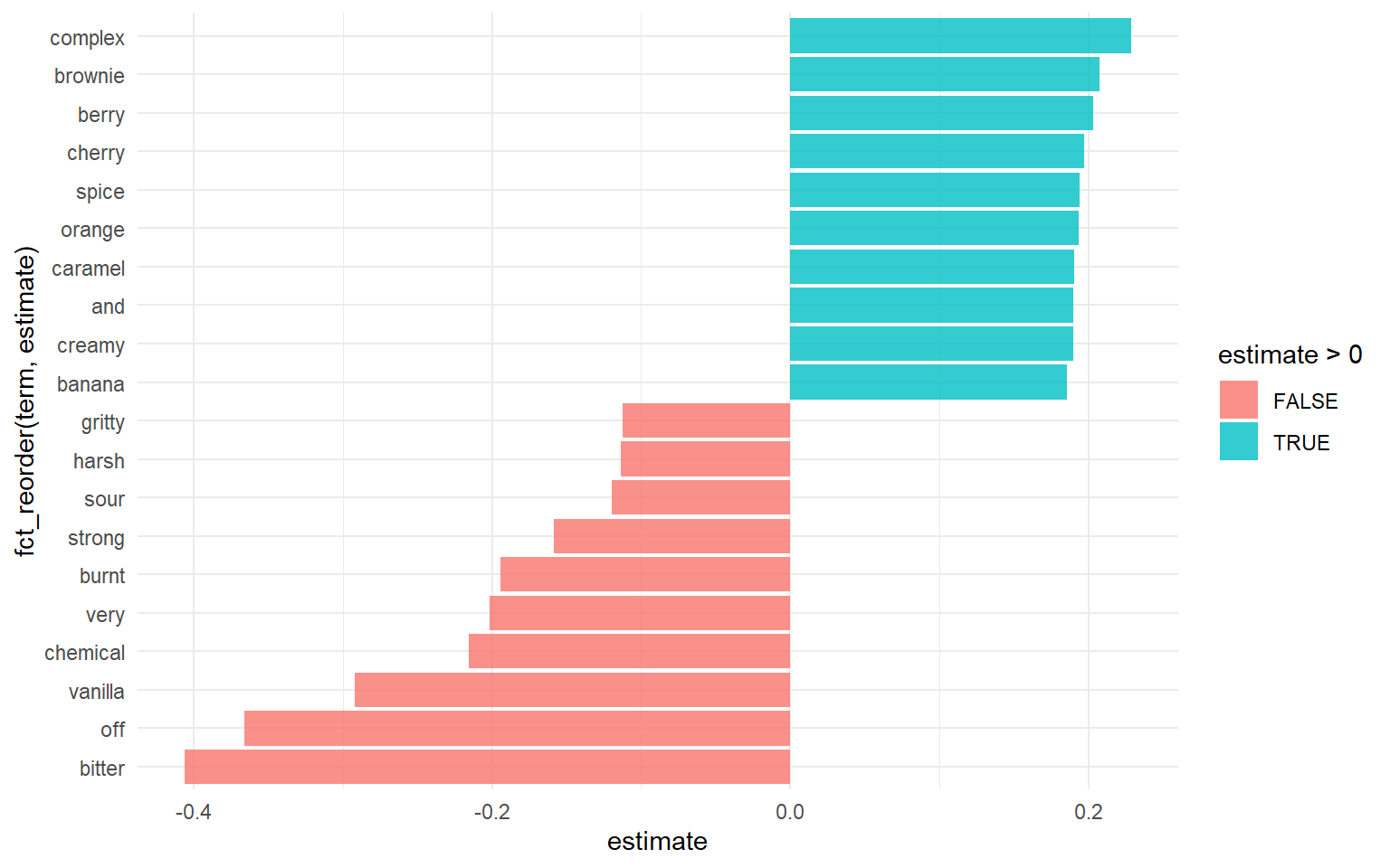
Here we can see words most commonly associated with good ratings, and bad ratings
extract_workflow(final_fitted) %>%
  tidy() %>%
  filter(term != "Bias") %>%
  group_by(estimate > 0) %>%
  slice_max(abs(estimate), n = 10) %>%
  ungroup() %>%
  mutate(term = str_remove(term, "tf_most_memorable_characteristics_")) %>%
  ggplot(aes(estimate, fct_reorder(term, estimate), fill = estimate > 0)) +
  geom_col(alpha = 0.8)