Bootstrapped Resampling Regression & Revenue Forecasting
By Alex Labuda
November 28, 2022

In this post, I’ll begin by visualizing marketing related time-series data which includes revenue and spend for several direct marketing channels.
I will fit a simple regression model and examine the effect of each channel on revenue.
In order to better understand the reliability of each coefficient, I will fit many bootstrapped resamples to develop a more robust estimate of each coefficient.
Lastly, I will create a forecasting model to predict future revenue. Enjoy!
library(modeltime)
library(timetk)
library(lubridate)

interactive <- FALSE
The Data
df <-
  read_csv(
    file = "data/marketing_data.csv"
  ) %>%
  mutate(
    date = mdy(date)
  )
Visualize the Data
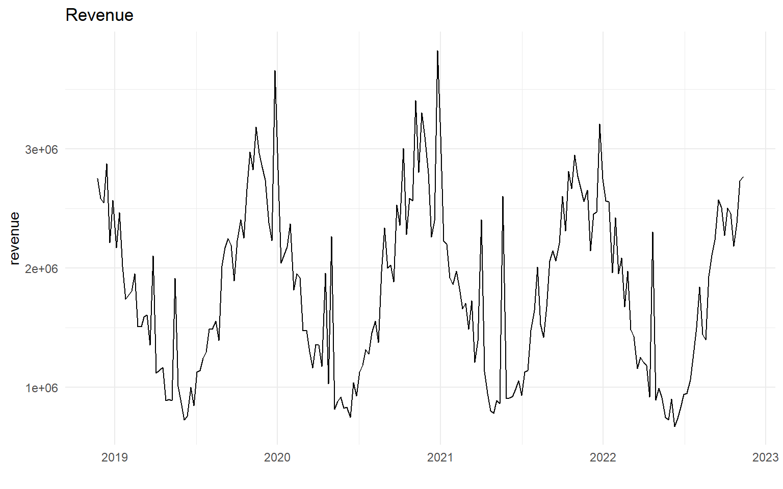
First lets visualize our target variable, revenue
df %>%
  ggplot(aes(date, revenue)) +
  geom_line() +
  labs(title = "Revenue",
       x = "")

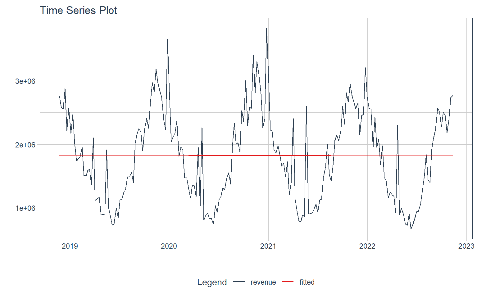
Fit: Simple Regression Model
First we’ll start by fitting a simple regression model to the data. This is just the grand mean of our data.
df %>%
    plot_time_series_regression(
        .date_var     = date,
        .formula      = revenue ~ as.numeric(date),
        .interactive  = interactive,
        .show_summary = FALSE
    )
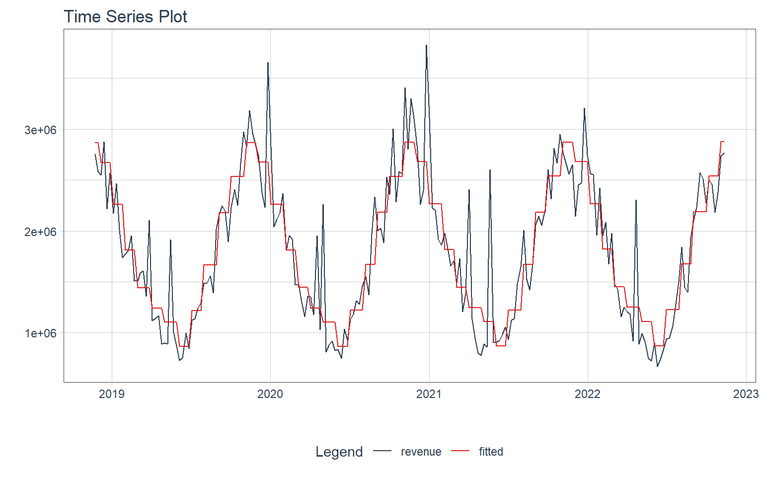
We can make a more accurate model by using month of year as independent variables for our model
df %>%
    plot_time_series_regression(
        .date_var     = date,
        .formula      = revenue ~ as.numeric(date) + month(date, label = TRUE),
        .interactive  = interactive,
        .show_summary = FALSE
    )
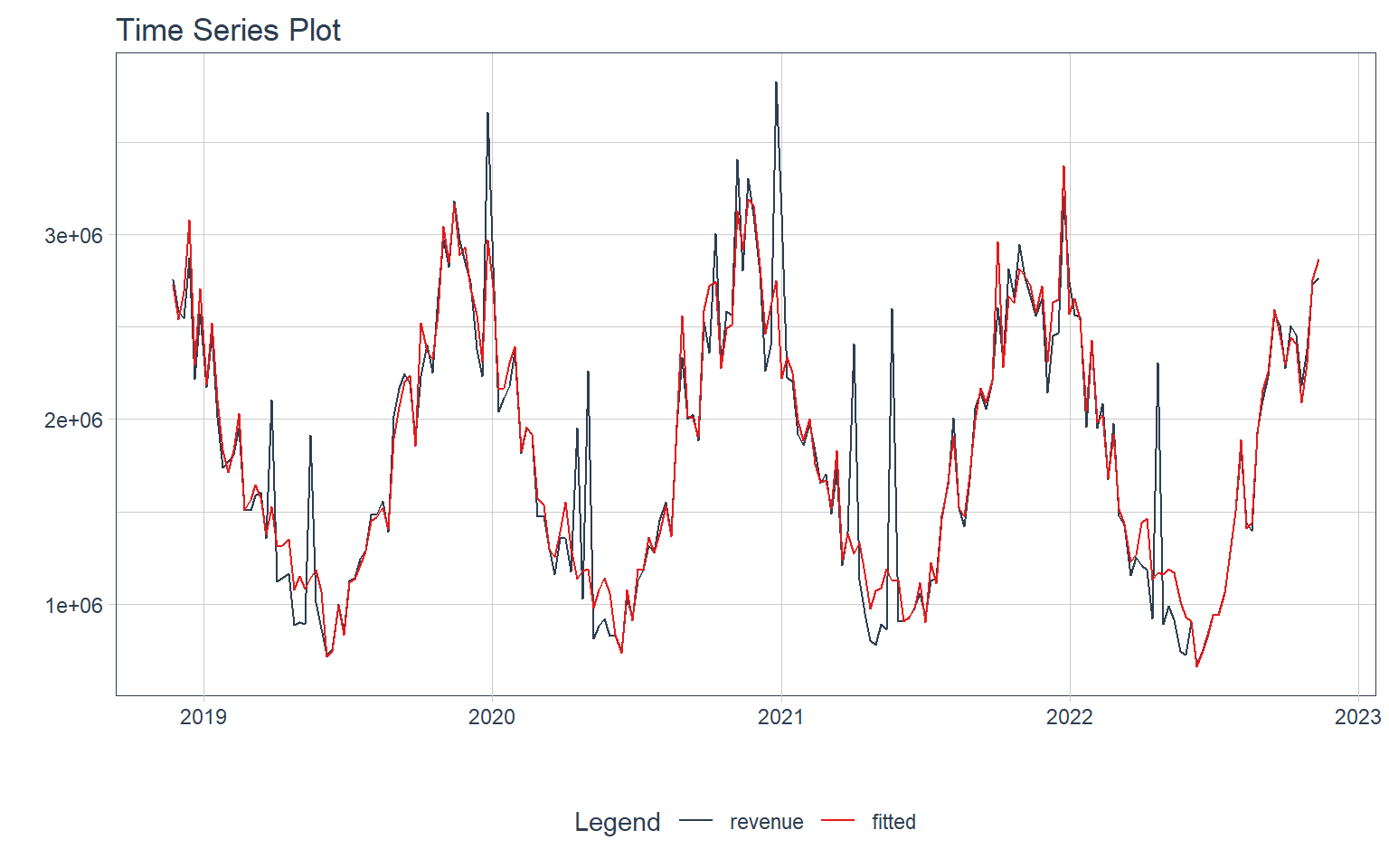
We can also introduce our spend variables as input to our model to study each channel’s effect on revenue
df %>%
    plot_time_series_regression(
        .date_var     = date,
        .formula      = revenue ~ as.numeric(date) + month(date, label = TRUE) + tv_spend +
          billboard_spend + print_spend + search_spend + facebook_spend + competitor_sales,
        .interactive  = interactive,
        .show_summary = FALSE
    )
A Simple Linear Model
Now lets take a look at our simple model output that includes direct marketing features and examine their effect of revenue
We can see that:
- TV spend, print spend, competitor sales and Facebook spend are statistically significant
- Print spend has the largest positive effect at increasing revenue of each of the direct marketing inputs
- A large positive intercept suggests that this company already has a strong baseline of sales
# forcing intercept to 0 to just show the gap from 0 instead of a base
revenue_fit <- lm(revenue ~ as.numeric(date) + tv_spend + billboard_spend + print_spend +
                    search_spend + facebook_spend + competitor_sales, data = df)
summary(revenue_fit)
##
## Call:
## lm(formula = revenue ~ as.numeric(date) + tv_spend + billboard_spend +
##     print_spend + search_spend + facebook_spend + competitor_sales,
##     data = df)
##
## Residuals:
##     Min      1Q  Median      3Q     Max
## -440321  -86030  -59261  -12997 1618906
##
## Coefficients:
##                    Estimate Std. Error t value Pr(>|t|)
## (Intercept)       7.345e+05  1.070e+06   0.687   0.4932
## as.numeric(date) -3.416e+01  5.754e+01  -0.594   0.5534
## tv_spend          5.007e-01  9.069e-02   5.521 1.04e-07 ***
## billboard_spend   4.183e-02  1.216e-01   0.344   0.7313
## print_spend       8.755e-01  3.950e-01   2.216   0.0278 *
## search_spend      5.364e-01  6.683e-01   0.803   0.4231
## facebook_spend    3.577e-01  2.095e-01   1.707   0.0893 .
## competitor_sales  2.868e-01  1.154e-02  24.846  < 2e-16 ***
## ---
## Signif. codes:  0 '***' 0.001 '**' 0.01 '*' 0.05 '.' 0.1 ' ' 1
##
## Residual standard error: 264700 on 200 degrees of freedom
## Multiple R-squared:  0.8681, Adjusted R-squared:  0.8634
## F-statistic:   188 on 7 and 200 DF,  p-value: < 2.2e-16
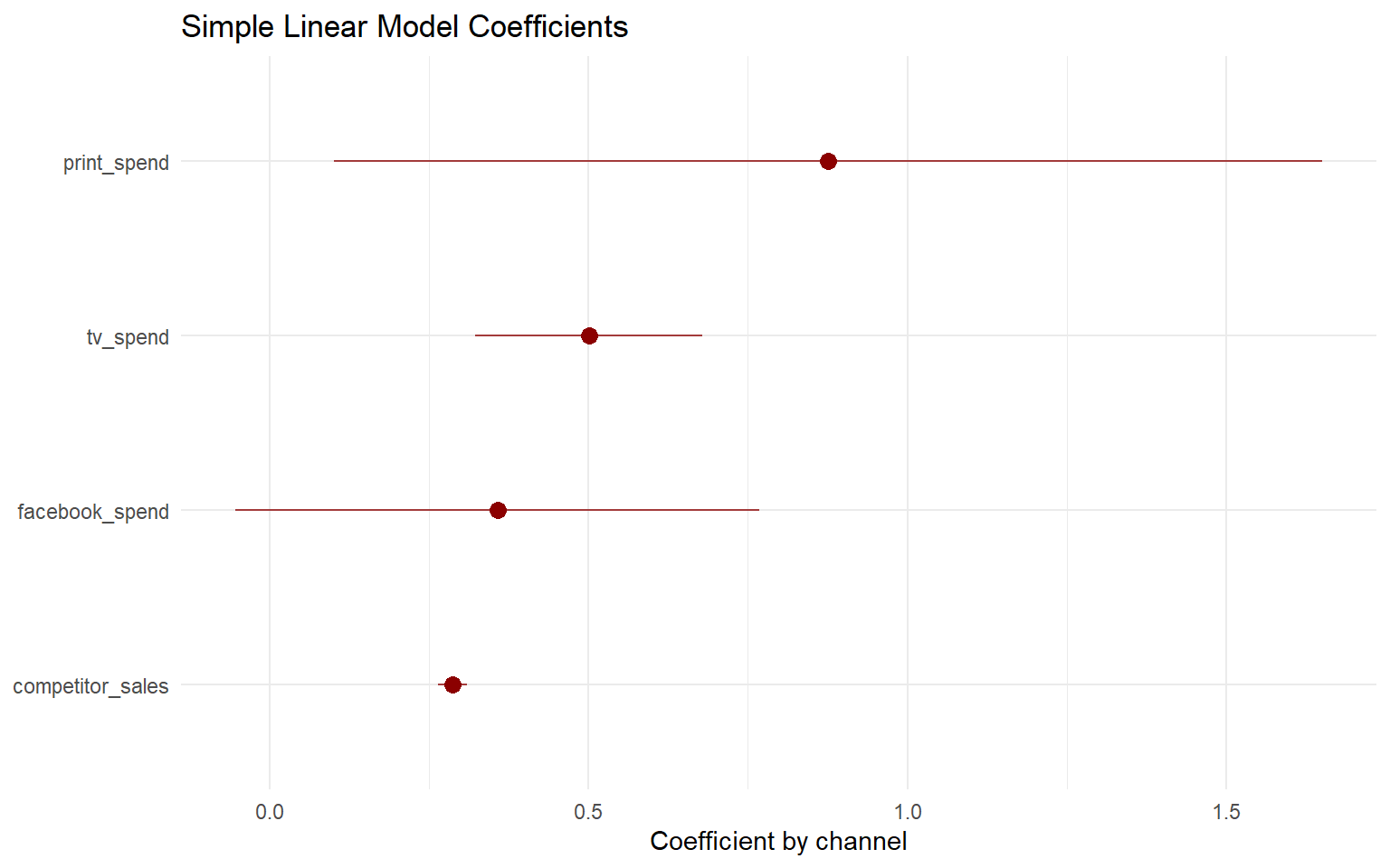
Viz: SLM coefficients
We can plot the coefficient and confidence intervals to make it easier to see the reliability of each estimate
- Print spend has the largest positive coefficient, but also the widest confidence interval
- Our model is very confident in the estimated effect of competitor sales
library(broom)
library(dotwhisker)

tidy(revenue_fit) %>%
  filter(p.value < 0.1) %>%
  mutate(
         term = fct_reorder(term, -estimate)) %>%
  dwplot(
    vars_order = levels(.$term),
    dot_args = list(size = 3, color = "darkred"),
  whisker_args = list(color = "darkred", alpha = 0.75)
  ) +
  labs(x = "Coefficient by channel",
       y = NULL,
       title = "Simple Linear Model Coefficients")
Fit: Bootstrap Resampling
How reliable are our coefficients?
We can fit a model using bootstrapped resamples of our data. This allows us to determine the stability of our coefficient estimates. Essentially this is fitting many small models to examine the variation of each channel’s coefficient.
- By default
reg_intervalsuses 1,001 bootstrap samples for t-intervals and 2,001 for percentile intervals.
library(rsample)

revenue_intervals <-
  reg_intervals(revenue ~ as.numeric(date) + tv_spend + billboard_spend + print_spend +
                    search_spend + facebook_spend + competitor_sales,
                data = df, keep_reps = TRUE)

revenue_intervals
## # A tibble: 7 × 7
##   term                .lower .estimate .upper .alpha .method         .replicates
##   <chr>                <dbl>     <dbl>  <dbl>  <dbl> <chr>     <list<tibble[,2]>
## 1 as.numeric(date) -138.      -35.1    64.7     0.05 student-t       [1,001 × 2]
## 2 billboard_spend    -0.123     0.0403  0.167   0.05 student-t       [1,001 × 2]
## 3 competitor_sales    0.263     0.287   0.304   0.05 student-t       [1,001 × 2]
## 4 facebook_spend     -0.0439    0.368   0.707   0.05 student-t       [1,001 × 2]
## 5 print_spend         0.263     0.875   1.42    0.05 student-t       [1,001 × 2]
## 6 search_spend       -0.639     0.575   1.71    0.05 student-t       [1,001 × 2]
## 7 tv_spend            0.199     0.513   0.763   0.05 student-t       [1,001 × 2]
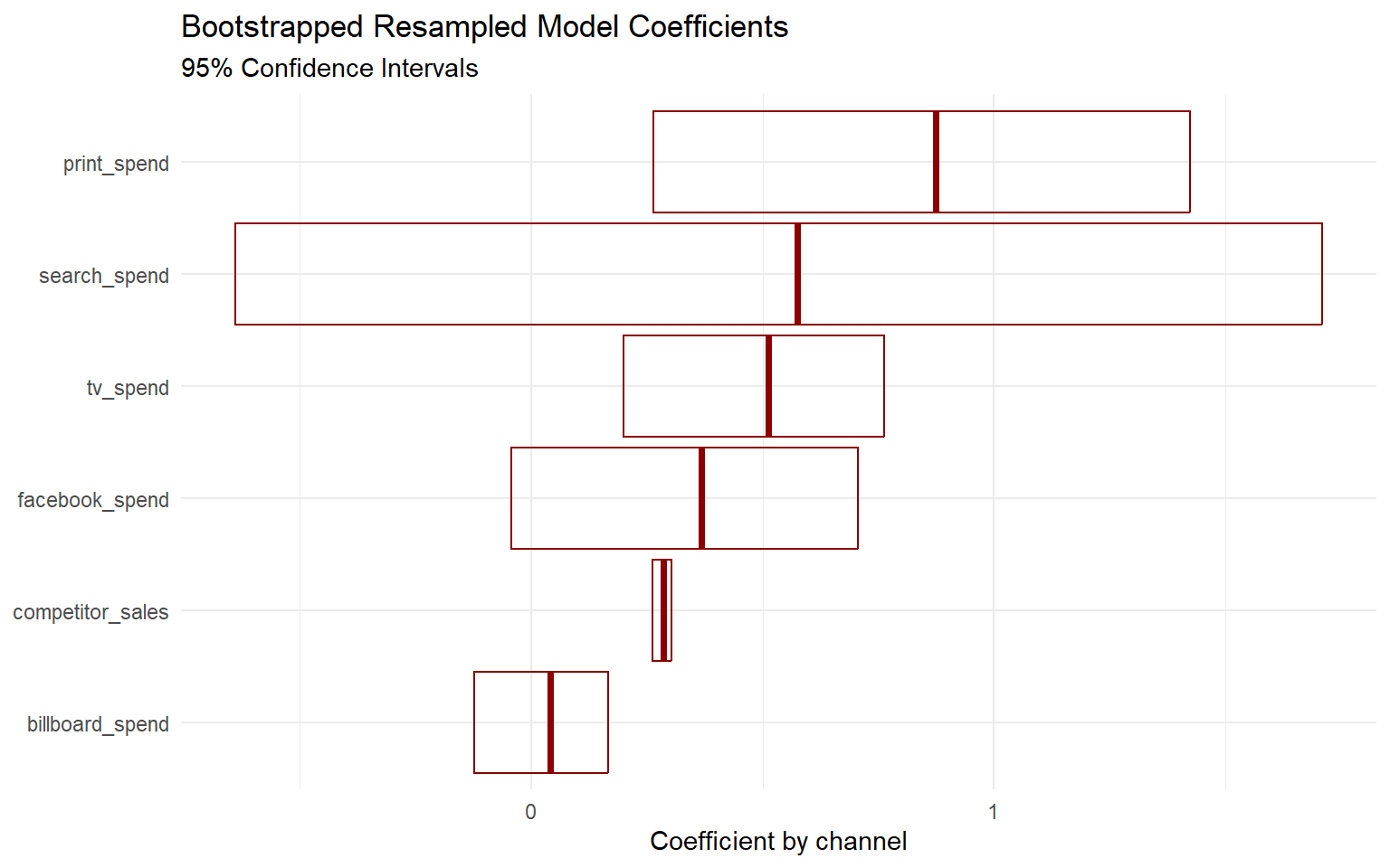
Viz: Bootstrapped Resampled Coefficients
Crossbar chart
- Here we can see the wide confidence interval surrounding
search_spend. - This makes sense since the coefficient for this channel in our first linear model was not statistically significant.
revenue_intervals %>%
  filter(!term == "as.numeric(date)") %>%
    mutate(
        term = fct_reorder(term, .estimate)
    ) %>%
    ggplot(aes(.estimate, term)) +
    geom_crossbar(aes(xmin = .lower, xmax = .upper),
                  color = "darkred", alpha = 0.8) +
  labs(x = "Coefficient by channel",
       y = NULL,
       title = "Bootstrapped Resampled Model Coefficients",
       subtitle = "95% Confidence Intervals")
Time-Series Forecasting
Lets build our forecasting model!
df_ts <-
  df %>%
  select(date, revenue)

df_ts %>%
  ggplot(aes(date, revenue)) +
  geom_line() +
  labs(title = "Revenue",
       x = "")
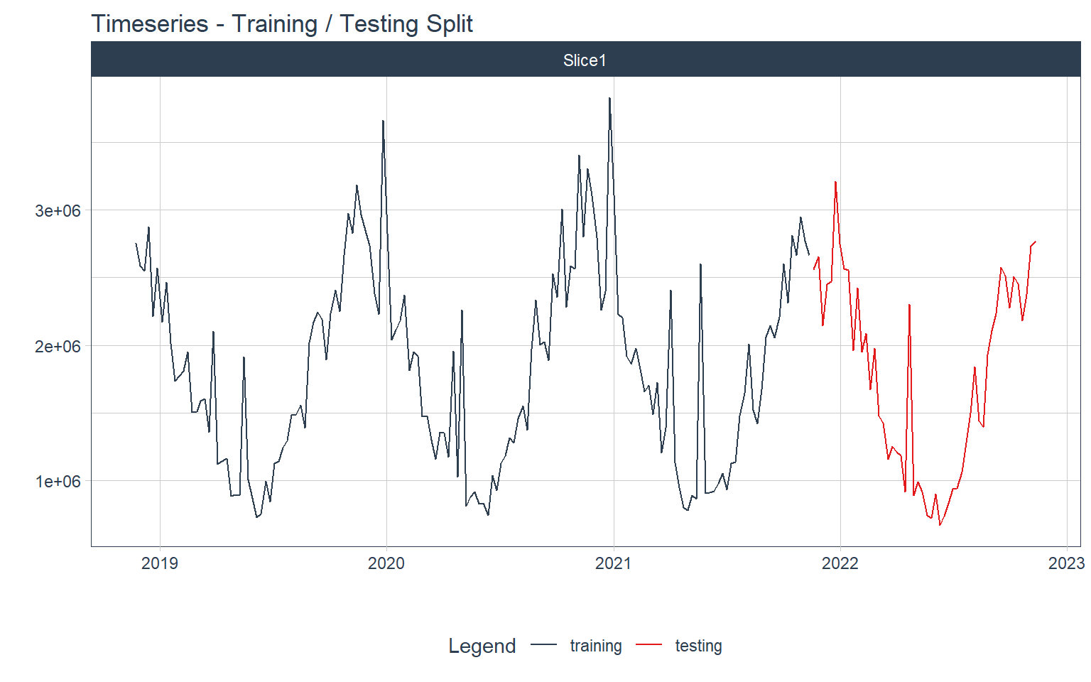
Training & Testing Splits
First, I’ll split the data into training and testing sets
splits <-
  df_ts %>%
  time_series_split(assess = "12 months", cumulative = TRUE)

splits %>%
  tk_time_series_cv_plan() %>%
  plot_time_series_cv_plan(date, revenue, .interactive = interactive) +
  labs(title = "Timeseries - Training / Testing Split")
Modeling
Now we can create the recipe for our model.
After we bake, we can see what the output looks like.
library(tidymodels)
recipe_spec_timeseries <-
  recipe(revenue ~., data = training(splits)) %>%
    step_timeseries_signature(date)

bake(prep(recipe_spec_timeseries), new_data = training(splits))
## # A tibble: 156 × 29
## date revenue date_in…¹ date_…² date_…³ date_…⁴ date_…⁵ date_…⁶ date_…⁷
## <date> <dbl> <dbl> <int> <int> <int> <int> <int> <int>
## 1 2018-11-23 2754372. 1.54e9 2018 2018 2 4 11 10
## 2 2018-11-30 2584277. 1.54e9 2018 2018 2 4 11 10
## 3 2018-12-07 2547387. 1.54e9 2018 2018 2 4 12 11
## 4 2018-12-14 2875220 1.54e9 2018 2018 2 4 12 11
## 5 2018-12-21 2215953. 1.55e9 2018 2018 2 4 12 11
## 6 2018-12-28 2569922. 1.55e9 2018 2018 2 4 12 11
## 7 2019-01-04 2171507. 1.55e9 2019 2019 1 1 1 0
## 8 2019-01-11 2464132. 1.55e9 2019 2019 1 1 1 0
## 9 2019-01-18 2012520 1.55e9 2019 2019 1 1 1 0
## 10 2019-01-25 1738912. 1.55e9 2019 2019 1 1 1 0
## # … with 146 more rows, 20 more variables: date_month.lbl <ord>,
## # date_day <int>, date_hour <int>, date_minute <int>, date_second <int>,
## # date_hour12 <int>, date_am.pm <int>, date_wday <int>, date_wday.xts <int>,
## # date_wday.lbl <ord>, date_mday <int>, date_qday <int>, date_yday <int>,
## # date_mweek <int>, date_week <int>, date_week.iso <int>, date_week2 <int>,
## # date_week3 <int>, date_week4 <int>, date_mday7 <int>, and abbreviated
## # variable names ¹date_index.num, ²date_year, ³date_year.iso, ⁴date_half, …
Preprocessing Steps
Now we’ll add a few additional preprocessing steps to our recipe:
- Convert a date column into a fourier series
- Remove date
- Normalize the inputs
- one-hot encode categorical inputs (add dummies)
recipe_spec_final <- recipe_spec_timeseries %>%
    step_fourier(date, period = 365, K = 1) %>%
    step_rm(date) %>%
    step_rm(contains("iso"), contains("minute"), contains("hour"),
            contains("am.pm"), contains("xts")) %>%
    step_normalize(contains("index.num"), date_year) %>%
    step_dummy(contains("lbl"), one_hot = TRUE)

recipe_spec_prophet <- recipe_spec_timeseries

juice(prep(recipe_spec_final))
## # A tibble: 156 × 39
##     revenue date_index…¹ date_…² date_…³ date_…⁴ date_…⁵ date_…⁶ date_…⁷ date_…⁸
##       <dbl>        <dbl>   <dbl>   <int>   <int>   <int>   <int>   <int>   <int>
##  1 2754372.        -1.71   -2.14       2       4      11      23       0       6
##  2 2584277.        -1.69   -2.14       2       4      11      30       0       6
##  3 2547387.        -1.67   -2.14       2       4      12       7       0       6
##  4 2875220         -1.65   -2.14       2       4      12      14       0       6
##  5 2215953.        -1.62   -2.14       2       4      12      21       0       6
##  6 2569922.        -1.60   -2.14       2       4      12      28       0       6
##  7 2171507.        -1.58   -1.01       1       1       1       4       0       6
##  8 2464132.        -1.56   -1.01       1       1       1      11       0       6
##  9 2012520         -1.54   -1.01       1       1       1      18       0       6
## 10 1738912.        -1.51   -1.01       1       1       1      25       0       6
## # … with 146 more rows, 30 more variables: date_mday <int>, date_qday <int>,
## #   date_yday <int>, date_mweek <int>, date_week <int>, date_week2 <int>,
## #   date_week3 <int>, date_week4 <int>, date_mday7 <int>, date_sin365_K1 <dbl>,
## #   date_cos365_K1 <dbl>, date_month.lbl_01 <dbl>, date_month.lbl_02 <dbl>,
## #   date_month.lbl_03 <dbl>, date_month.lbl_04 <dbl>, date_month.lbl_05 <dbl>,
## #   date_month.lbl_06 <dbl>, date_month.lbl_07 <dbl>, date_month.lbl_08 <dbl>,
## #   date_month.lbl_09 <dbl>, date_month.lbl_10 <dbl>, …
Model Specs
- linear regression
- xgboost
model_spec_lm <- linear_reg(mode = "regression") %>%
    set_engine("lm")

model_spec_xgb <- boost_tree(mode = "regression") %>%
  set_engine("xgboost")

model_spec_prophet <- prophet_reg(mode = "regression") %>%
  set_engine("prophet")
Workflow
We can add our recipe and model to a workflow
workflow_lm <- workflow() %>%
    add_recipe(recipe_spec_final) %>%
    add_model(model_spec_lm)

workflow_xgb <- workflow() %>%
  add_recipe(recipe_spec_final) %>%
  add_model(model_spec_xgb)

workflow_prophet <- workflow() %>%
  add_recipe(recipe_spec_prophet) %>%
  add_model(model_spec_prophet)
Fit our Model
workflow_fit_lm <-
  workflow_lm %>%
  fit(data = training(splits))

workflow_fit_xgb <-
  workflow_xgb %>%
  fit(data = training(splits))

workflow_fit_prophet <-
  workflow_prophet %>%
  fit(data = training(splits))
model_table <- modeltime_table(
  workflow_fit_lm,
  workflow_fit_xgb,
  workflow_fit_prophet
)

calibration_table <- model_table %>%
  modeltime_calibrate(testing(splits))
Measure Accuracy
calibration_table %>%
    modeltime_accuracy(acc_by_id = FALSE) %>%
    table_modeltime_accuracy(.interactive = FALSE)
| Accuracy Table | ||||||||
| .model_id | .model_desc | .type | mae | mape | mase | smape | rmse | rsq |
|---|---|---|---|---|---|---|---|---|
| 1 | LM | Test | 242994.3 | 16.19 | 0.90 | 15.14 | 313485.5 | 0.80 |
| 2 | XGBOOST | Test | 260391.4 | 18.67 | 0.97 | 16.33 | 352541.8 | 0.76 |
| 3 | PROPHET W/ REGRESSORS | Test | 306623.9 | 21.62 | 1.14 | 18.85 | 384166.2 | 0.79 |
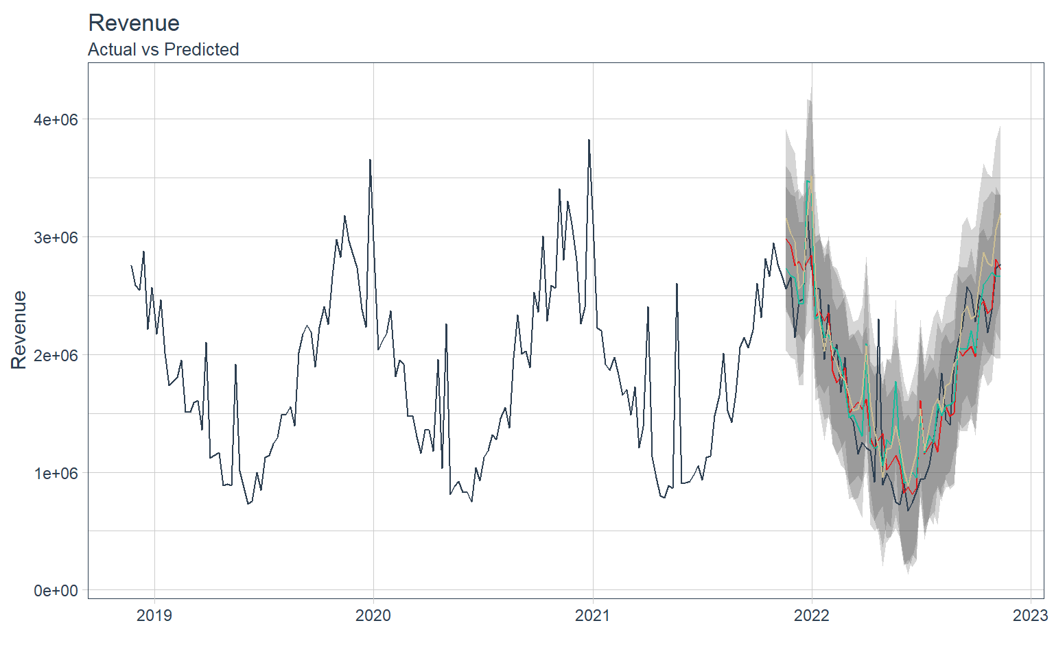
Forcasting Results
Lets visualize each model’s prediction accuracy
calibration_table %>%
  modeltime_forecast(actual_data = df_ts) %>%
  plot_modeltime_forecast(.interactive = FALSE) +
  labs(
    y = "Revenue",
    title = "Revenue",
    subtitle = "Actual vs Predicted"
  ) +
  theme(legend.position = "none")
Sources: Matt Dancho, Julia Silge
- Posted on:
- November 28, 2022
- Length:
- 8 minute read, 1641 words